Gaining Insights into a Mechanical Model with Decision Trees

Link zur deutschen Version: Mit Entscheidungsbäumen Einblick in ein mechanisches Modell gewinnen

---

In this post, I would like to present how to use decision trees to gain insight into an existing model. 

This blog already contains several posts on applications for artificial intelligence (AI) and, more specifically, machine learning (ML) in the civil engineering domain (AI-augmented Structural Engineering, AI-assisted strut-and-tie models, ML-enhanced finite element analysis and the use of neural networks within the direct stiffness method). In comparison, this post contains a much smaller, simpler application, intended for readers who do not have previous knowledge in machine learning yet.

One of the main advantages of decision trees is that they are fairly easy to implement with little coding experience and no machine learning experience. This makes them particularly suitable as an entry point into machine learning. Conjunctly, the results are easy to interpret as they can be graphically represented as an intuitively understandable tree. In this post, I will use this property of decision trees to gain a deeper understanding of an existing model, in the example a mechanical model that calculates the load-bearing capacity of a continuous slab strip.

Some background

Machine learning, a sub-field of artificial intelligence, encompasses several methods to describe and learn from large amounts of data. To counteract its most prevalent disadvantage of users being unable to comprehend how and why the ML algorithm reached a certain result (black box model), research in the engineering domain has been focusing on explainable AI. Explainable AI algorithms are those whose predictions can be judged for plausibility and accuracy or even retraced with domain knowledge. A comprehensive review of explainable AI can be found in this open-source paper.

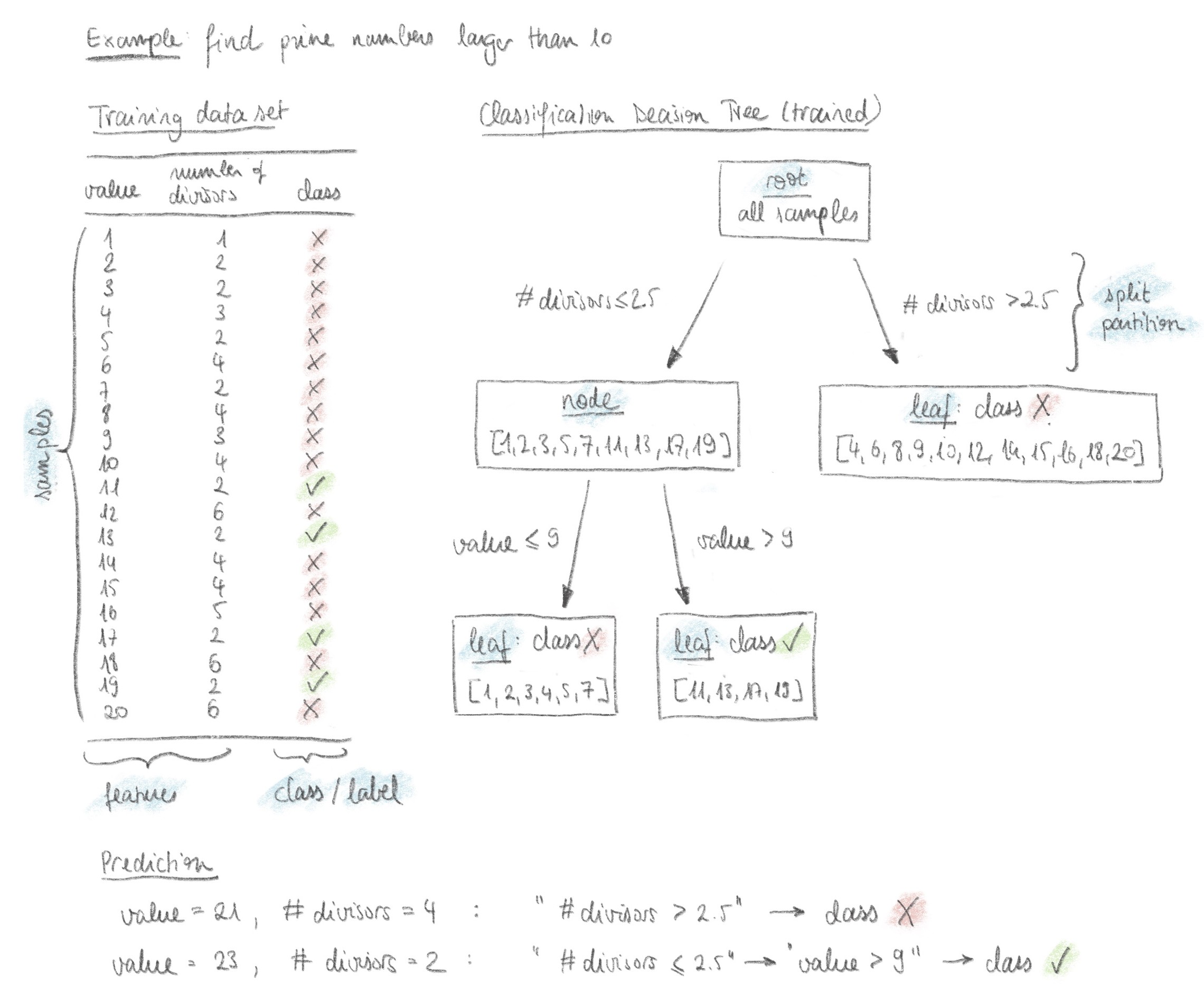
One of the simplest and most explainable machine learning algorithms is the (classification) decision tree. It is an algorithm that learns to predict a value (often the answer “yes” or “no”) by successively partitioning the input data based on certain input parameters (the features). The decision process can be visualised as a tree, branching at each partition. Given that each partitioning step can be evaluated by the user, the model’s outcome is very explainable. Figure 1 shows the example of a decision tree that classifies numbers into the classes “prime number > 10” and “not a prime number > 10”, given the features of each number’s value and number of divisors. During training with the data set on the left, the algorithm finds the best partitions. The trained decision tree can then be used to predict the class of new samples. The Jupyter notebook with the code of this example can be found in this github repository.

Application example

The following example demonstrates how to use a decision tree classifier to gain insight into an existing mechanical model. The focus is not, as usual and shown in the previous simple example, on finding the most accurate classification model to predict the class of new data, but on understanding which partitions the decision tree makes to reach the result. This can help gain insight into which parameters are most relevant for the outcome of the mechanical model.

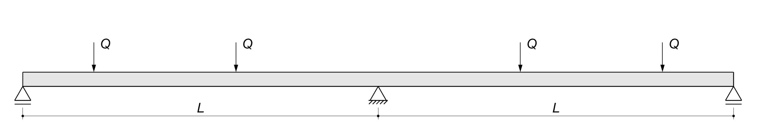
Consider the example of a continuous reinforced concrete slab strip (Figure 2). An existing mechanical model, validated with large-scale experiments, calculates the non-linear response of the slab strip and can predict its ultimate load, taking into account the limited deformation capacity of the used materials. It is of interest to know which parameter combinations lead to a load-bearing capacity higher than the limit load calculated according to the Theory of Plasticity¹It is possible to reach load-bearing capacities higher than the limit load with the mechanical model because it takes into account the hardening behaviour of the reinforcing steel, whereas the yield stress is used when calculating the limit load according to the Theory of Plasticity.. This means that in that configuration, the used materials have a deformation capacity high enough to use simplified calculation methods according to the Theory of Plasticity safely. More background on this topic can be found for example in this blog post.

The decision tree will be trained to predict a class of “ok” if the load-bearing capacity calculated by the non-linear mechanical model exceeds the limit load (Q_u/Q_pl > 1) or “not ok” otherwise.

Creation of the data set

A data set can be generated by running the mechanical model many times with different input parameters. Choosing the correct parameters, or features in ML terminology, is one of the most crucial steps in data generation. The data set could look as follows:

fs [MPa]	k [-]	εsu [-]	c [-]	ρs [%]	L [m]	fc [MPa]	Class
496	1.09	0.087	0.11	0.78	4.37	54.1	ok
505	1.13	0.026	0.06	2.94	4.53	41.7	not ok
483	1.13	0.092	0.25	0.51	7.12	36.4	ok
517	1.07	0.082	0.08	0.88	4.37	57.8	ok
491	1.11	0.081	0.18	1.74	6.61	29.0	not ok
…	…	…	…	…	…	…	…

Notations

f_s: Yield stress of the reinforcing bars

k: hardening ration of the reinforcing bars (k = f_s/f_t, where f_t = tensile strength of the reinforcing bars)

ε_su: strain at the tensile strength of the reinforcing bars

c: “roundness” of the constitutive material law of the reinforcing bars, see parameter c₃ in “S. Haefliger, K. Thoma, and W. Kaufmann, ‘Influence of a triaxial stress state on the load-deformation behaviour of axisymmetrically corroded reinforcing bars’, Construction and Building Materials, vol. 407 (Link) 

ρ_s: reinforcement ratio at the intermediate support (the reinforcement ratio in the span is calculated according to the linear elastic bending moment profile)

L: span width of the continuous beam

f_c: compressive strength of the concrete

It is good practice to set the problem up such that the classes are balanced, i.e. an approximately equal number of samples per class, otherwise the algorithm is prone to favour the stronger classes.

Creation of the decision treeThe decision tree classifier can be created, using, for example, an implementation from the open-source Python library scikit-learn. Important parameters (called hyperparameters in machine learning) are the maximum depth of the tree and the minimum number of samples per leaf (end node). These hyperparameters help prevent overfitting of the data, as discussed later.

Training the decision tree

The training process starts at a root node containing the entire data set. The data is then partitioned using for example the Gini impurity criterion. For various possible features and split values, the algorithm calculates the Gini impurity to find the split that best minimizes impurity. This means identifying the feature and value that best separates the data into pure subsets. The algorithm creates a new level of nodes and continues on this level. This process is repeated until the maximum tree depth is reached or the number of samples in a node is too small to split further (i.e. the minimum number of values per leaf is reached). The performance of the decision tree is then evaluated to ensure its predictions are accurate enough for interpretation. This article provides an overview of methods for the performance evaluation.

Interpretation of the results

The most convenient way to interpret the results is by using a graphical representation of the tree, such as the function included in scikit-learn or dtreeviz. This is, of course, only possible up to a certain tree depth, after which is becomes unwieldy. Figure 3 shows an example of a tree with depth 3, though decision trees with different hyperparameters trained on the same data set were also analysed.

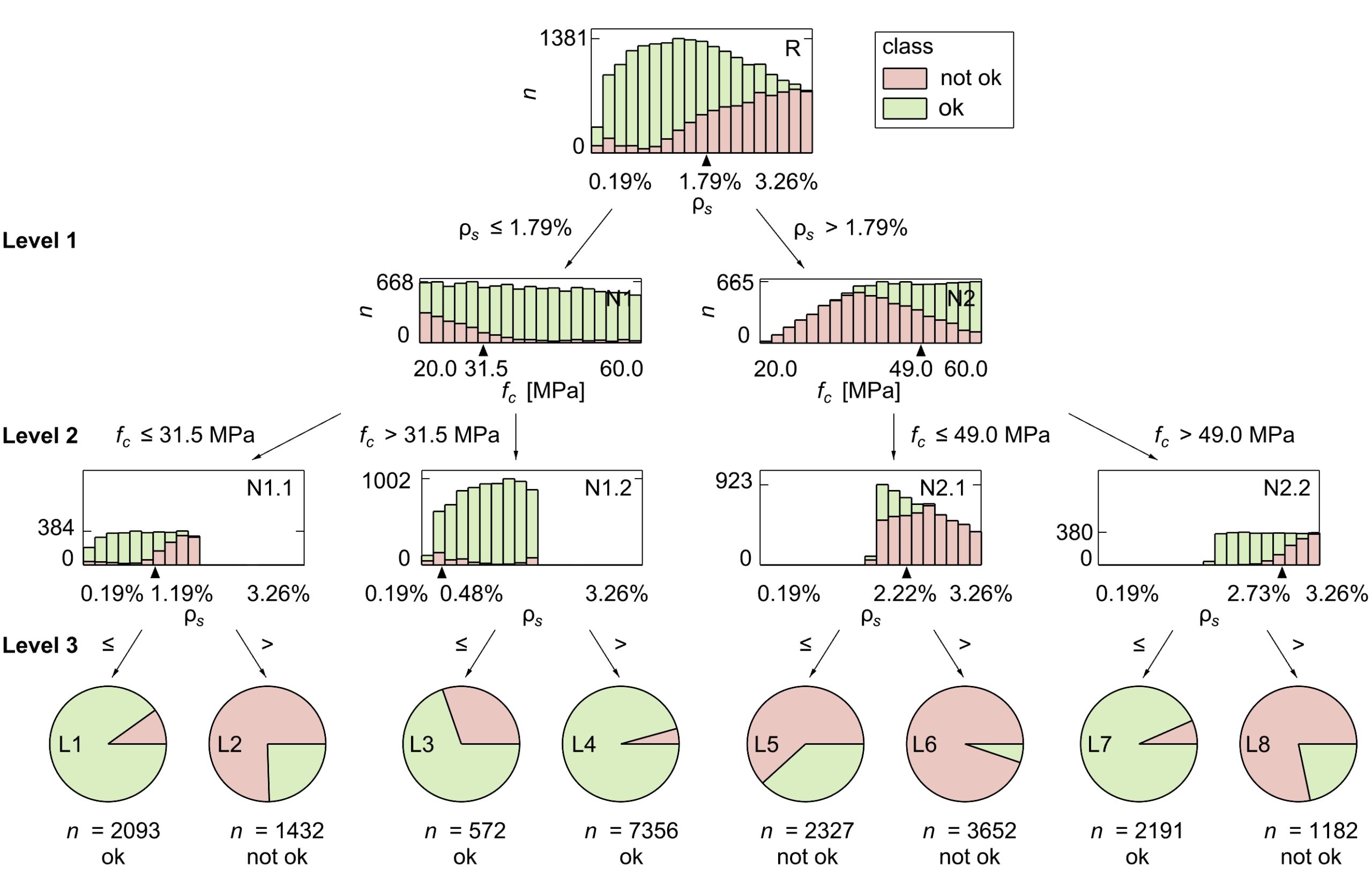
The partitions in the resulting tree can be interpreted with domain knowledge. In the application example, the first partition always (i.e. for all analysed tree depths) splits the data at a reinforcement ratio close to 1.8% (see Figure 3, Level 1). This indicates a meaningful relationship within the data. 

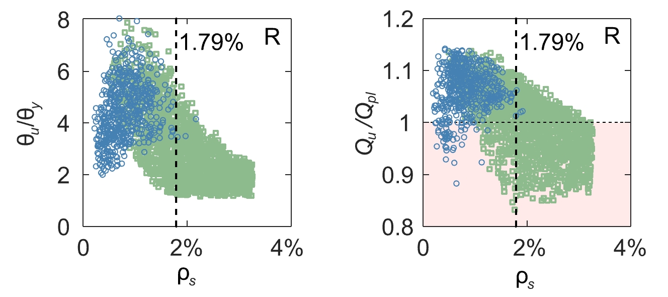
Some background on the failure criteria in each section of the mechanical model helps interpret this relationship. The cross-section can fail either by rupture of the reinforcement or if the concrete in the compression zone reaches a nominal strain, set to indicate failure by concrete crushing. Following the graphical representation used in this blog post, it becomes clear that the algorithm separates the data according to the failure mode, see Figure 4. This is remarkable, considering the data contains no information on the failure mode (see Table 1) and speaks for its importance in the mechanical model.

The second level of partitions is slightly less intuitive, as none of the failure criteria directly depend on the concrete compressive strength f_c²Failure by steel rupture if the steel strain in any section exceeds the ultimate steel strain ε_su. Failure by concrete crushing if the mean concrete strain at the compressed edge of the cross-section exceed 5‰, independently of the concrete compressive strength.. Plotting the data with the mechanical reinforcement ratio ω on the abscissa shows a clearer picture. The concrete compressive strength is part of the definition of the mechanical reinforcement ratio.

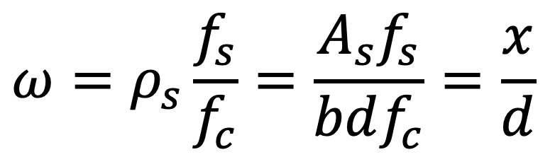
Notations

ω: mechanical reinforcement ratio

ρ_s: reinforcement ratio 

f_s: Yield stress of the reinforcing bars

f_c: compressive strength of the concrete

A_s: Cross-sectional area of the reinforcing bars

b: width of the cross-section

d: static depth

x: distance to neutral axis / depth of the compression zone

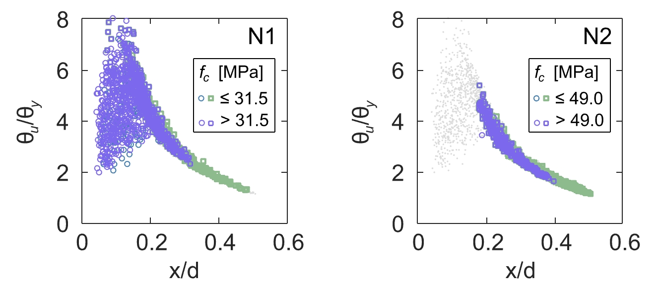
This ratio is known to have a significant influence on the ductility of structures. It is included in the Swiss and European codes with the condition x/d < 0.35 that needs to be fulfilled in order to use plastic methods in design. Interpreting the partition from the mechanical point of view, a high concrete compressive strength reduces the depth of the compression zone x, favouring reinforcement rupture as a failure mechanism and large rotations at failure θ_u (i.e. high rotation capacity, high ductility).

A high concrete compressive strength f_c keeps the ratio low, and the higher the reinforcement ratio ρ_s, the higher f_c needs to be to counteract it. This may explain the different split values f_c = 31.5 MPa and f_c = 49.0 MPa at the branches of Level 2, see Figure 3 and Figure 5. 

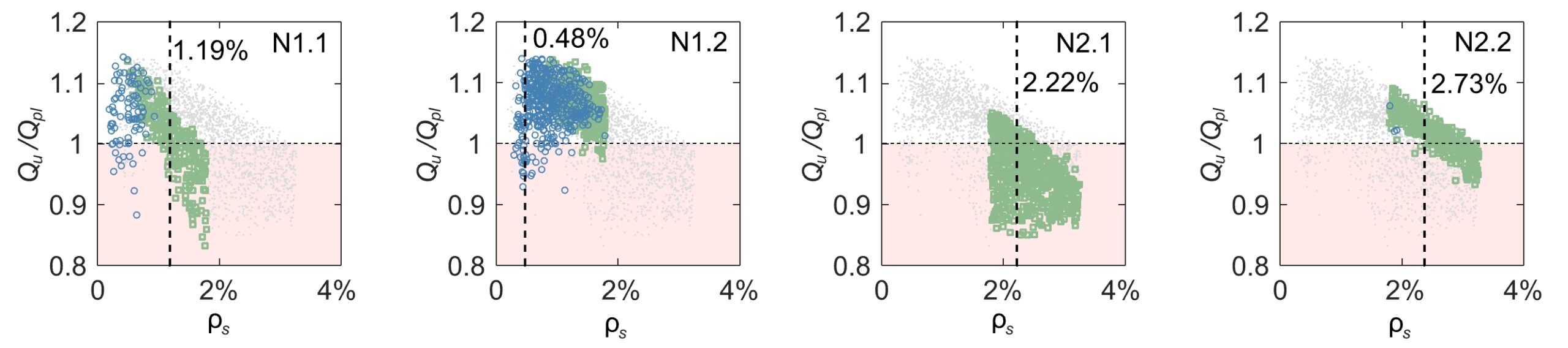
On Level 3 (see Figure 3 and Figure 6), the data is partitioned along the reinforcement ratio ρ_s again, solidifying the assumption that this is one of the most important design variables. Note that it is not usual for all nodes at the same level to be partitioned along the same variable. When interpreting the partitions, it is also important to consider their accuracy. In leaf L5, the decision tree misclassifies nearly 40 % of the samples, see Figure 3. Taking the accuracy into account, the interpretation of node N2.1 should be that samples with ρ_s > 2.22% are very likely “not ok”, but in the case of ρ_s < 2.22%, at least one additional level is required to separate the data well.

To summarize, creating a decision tree from data generated with the existing mechanical model and analysing the different partitions has (i) helped gain insight into what the most important features are and (ii) created an incentive to uncover the relation between these features and well-known mechanical principles. 

Limitations of the method 

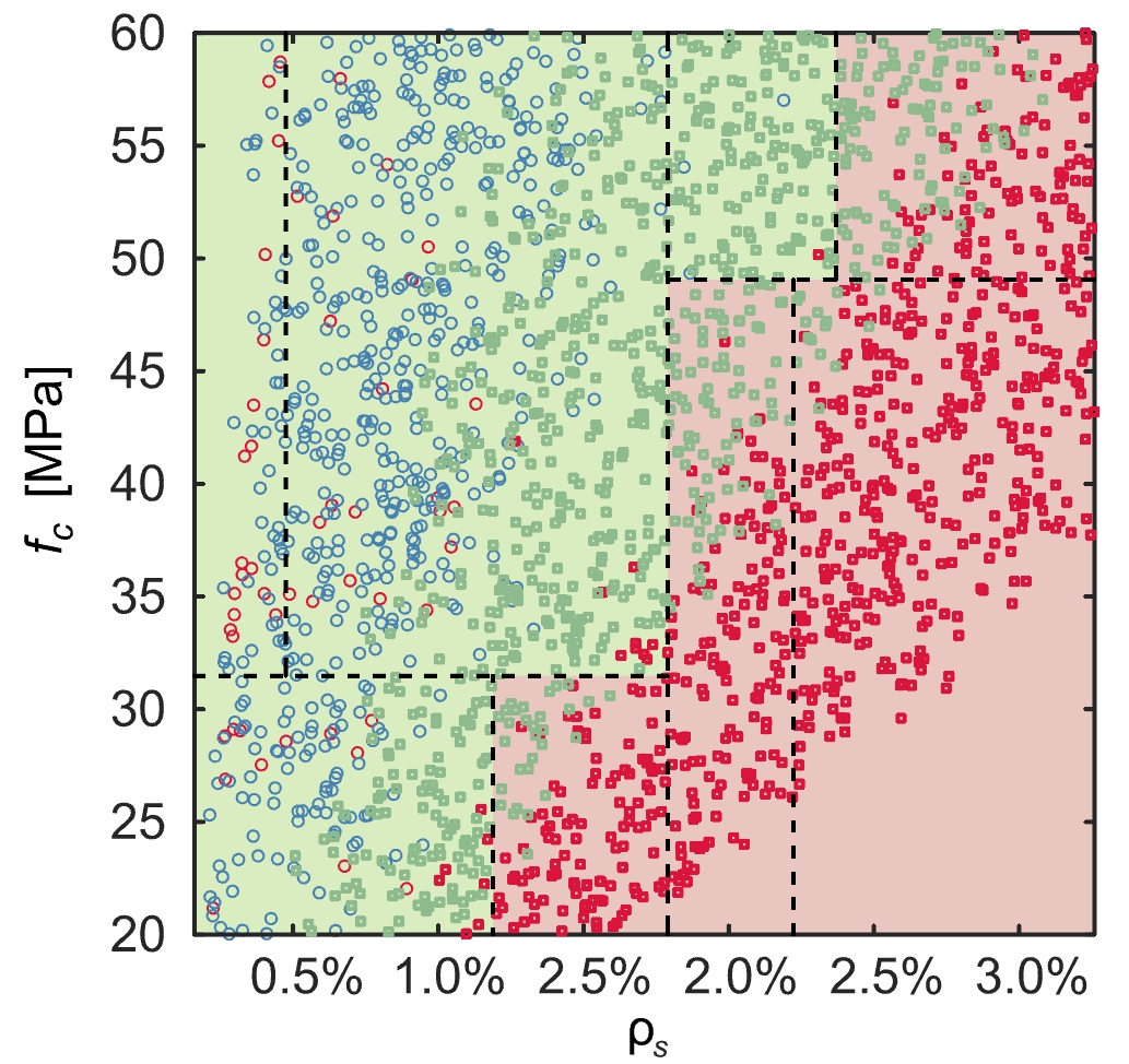
As mentioned, the results are only easily interpretable up to a certain tree depth, limiting its applicability to very complex problems. The approach is only simple for (one) categorical questions with few answers, as seen in the application example. Furthermore, the fact that the decision tree can only split the data set along one design variable in each partition (see Figure 7 for an illustration in 2 dimensions) may limit its application to complex, non-linear problems with many dependent design variables.

If the maximum tree depth is set too high or the minimum number of samples per split or per leaf are set to low, the decision tree might overfit, singling out certain points. This makes the fitted decision tree less generalisable and undermines the physical interpretability. A good way to check if the decision tree is overfitting is separating the data set into a training set and a test set. The decision tree is trained on the training data set without ever seeing the test data set. If the decision tree performs significantly worse when predicting the class of the test set compared to the training set, this is a good indication that it is overfitting. This article gives an overview of some methods to prevent or mitigate overfitting.

Decision trees rely on a balanced data set (i.e. with a similar number of samples per class), or they will favour the more represented class. This issue can be mitigated by introducing weighting factors, though they create an issue of their own, attributing overdue importance to outliers. If the weighting factor of the less represented class is five times the weighting factor of the more represented class, the tree could create a leaf with one outlier of the less represented class and four valid samples of the more represented class and still predict the less represented class in that leaf. This can only be noticed by carefully checking the plausibility of the partitions leading to each leaf. It is thus preferable to create balanced data sets or, if possible, remove outliers before training the decision tree.

Like all ML models, the outcome of decision trees depends heavily on the data. One should be aware that small changes in the data or the hyperparameters can lead to a different tree. As decision trees can be trained quickly, it is recommended to vary the hyperparameters and check that the trees and their interpretation remain similar. 

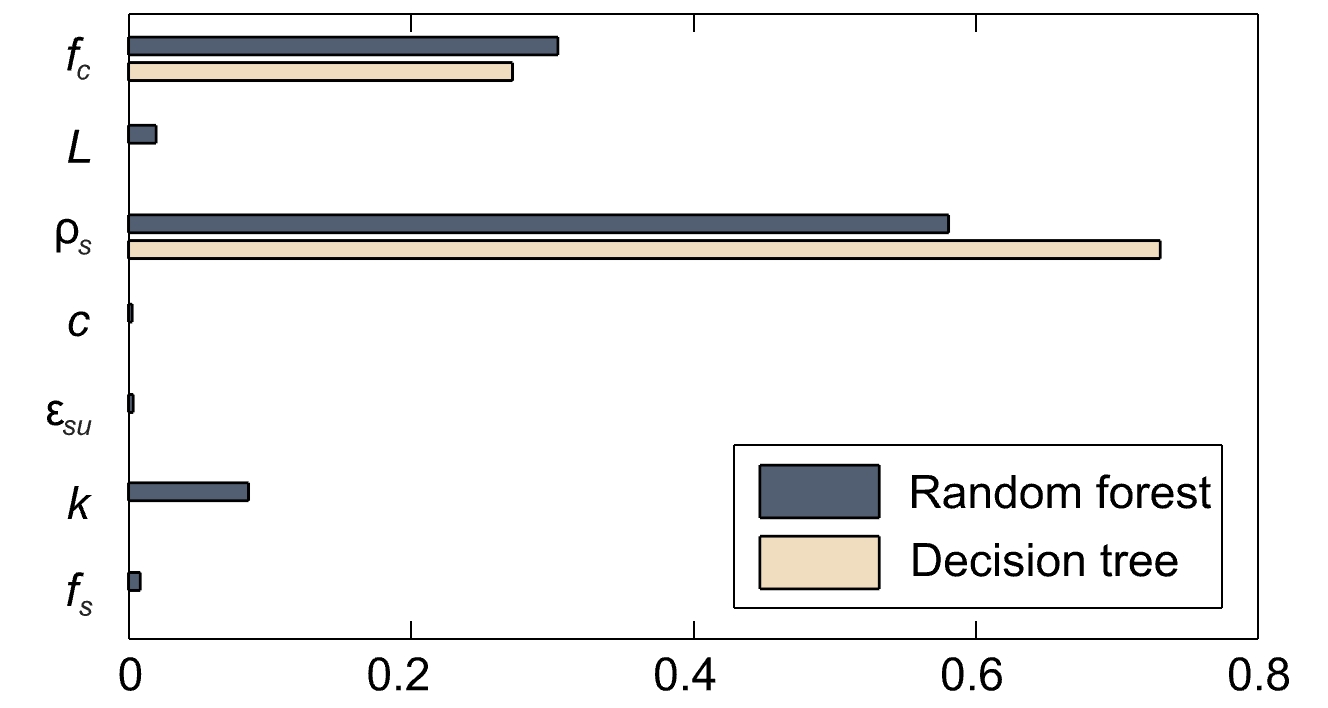
If the decision tree is not accurate enough, one could instead use a random forest algorithm, which generates multiple decision trees during training and provide the majority decision of these trees for a given dataset and given hyperparameters. It can represent complex data sets more accurately and is more robust against overfitting (see this article for a comparison). However, this comes at the cost of explainability as the large number of generated decision trees makes it impractical to manually interpret them all. With random forests, it is thus more convenient to use the relative importance of the features for interpretation, see Figure 8.

Personal assessment

Despite the limitations, I think using a decision tree on data generated by an existing model is an interesting approach because one can get a better understanding of the model and the data with little effort. The process helped me avoid getting overwhelmed by the high dimensionality (many features) in the mechanical model since the decision tree gave some indications on which ones to focus on. It also had the benefit of sparking my creativity and making me think about the problem differently when the results did not immediately align with my expectations. This led me to delve deeper into my preliminary theoretical knowledge of the problem and ultimately to a deeper understanding of the mechanical model. 

Resources

This github repository contains a short guide to get started with decision trees (using the sklearn toolbox and Visual Studio Code) and the Jupyter notebook with the code for the decision tree example in Figure 1 (prime numbers). 

---

Nathalie Reckinger