Link zur deutschen Version: Einblick in die Deep Neural Network Direkt Stiffness Methode (DNN-DSM)
This blog post describes the most important steps that were done throughout the development of the deep neural network direct stiffness method (DNN-DSM). The overall conceptual method derivation is basically separated into three parts: (i) the finite element simulation and development of appropriate data sets, based on local shell-element simulations, covering for instabilities at the cross-sectional level; (ii) the development of deep neural networks, suitable to predict the individual tangent stiffnesses; (iii) the implementation into the direct stiffness method.
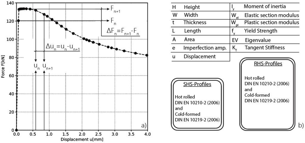
The developed deep neural network (DNN) models were trained on data sets derived from a pool of numerical LBA (linear buckling analysis) and GMNIA (geometrically and materially nonlinear analysis with imperfections) shell FE-simulations, designed in such a way that only local buckling is the main instability phenomena for the investigated rectangular and squared (RHS and SHS) cross-sections, see Figure 1.
The main verification work against experimental tests goes back on the Hollosstab project (Link). The derived FE-models were partially adapted based on this investigation and were further developed to match the conditions for local buckling. The developed FE-models are described as follows; (i) Abaqus Type S4R elements, with a mesh density of around 60 elements in circumferential and 50 – 100 elements per meter in longitudinal direction; (ii) Geometry based on code provisions of EN 10210-2:2006 and EN 10219-2:2006, with a length L set as the bigger value of the width W or the height H ; (iii) Deformations applied through defined reference points located at the upper and lower edge of the cross-section, connected through multiple point constraints (MPC-Pin formulation); (iv) Non-linear material models for hot-rolled (bilinear + non-linear model) and cold-formed steel (two-stage Ramberg Osgood model); (v) LBA analysis carried out to identify elastic critical buckling resistance and the eigenshape (local imperfections); (vi) GMNIA simulation performed to determine the realistic buckling resistance.
526 European hot rolled and cold-formed RHS and SHS profiles, three different steel grades ranging from mild to high-strength (S355, S460 and S700), as well as three different local imperfection amplitudes (B/200, B/300 and B/400; where B is the smaller dimension of either the profile height or width were taken into account. In sum, 9468 GMNIA simulations were run to create the basis for data extraction.
Therefore, the LBA analysis output from Abaqus was used to extract the cross-section-dependent elastic critical buckling load. The GMNIA analysis results, on the other hand, were used to determine the incremental deformation and rotation steps and an associated differential force and moments, see Figure 2 a) for compression. These values were subsequently used to calculate the incremental tangent stiffness values on which the DNN models were trained.
A total of 193 individual hyperparameter combinations for different DNN models were tested within the framework of preliminary investigations using the Random Search Method. This workflow was suitable in order to detect the overall tendencies within the DNN architecture. All calculations were performed on the basis of a train and test philosophy, meaning that a specific data amount was used for the training (80%) and an additional independent amount for the validation process (20%). The subsequent DNN model was built with four hidden layers (27, 27, 18, and 9 neurons), each ending with a ReLU activation function, a learning rate of 0.0005, and the Adam optimizer.

The general implementation of the DNN-DSM is based on the generic definition of the DSM for beam elements.
![]()
The DNN-DSM makes use of this implementation to predict a local nonlinear tangent stiffness matrix according to given nodal deformations or rotations. The neural network takes some of the features from Figure 2 b), as well as an absolute deformation or rotation at every step (see Figure 3 a) for compression and b) for bending) to predict a local nonlinear tangent stiffness matrix, as proposed through following equation.
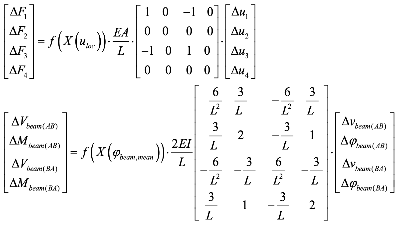
Implementing the beam element differs slightly from implementing the truss element by modifying the beam stiffness matrix according to a given mean rotation φ. The corresponding definition of the rotation φ for an element is stated in Figure 3 b). Therefore, an equal constant rotation at both ends is assumed, which is accurate enough as long as the element length remains small.
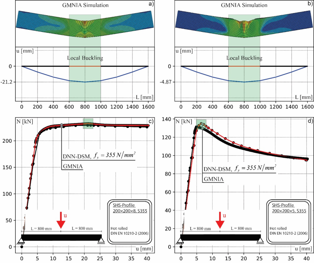
Three-point bending results are presented in Figure 4 for two hot-rolled profiles, SHS200x8 (S355) and SHS200x5 (S355). Figure 4 a) and b) show the output deformations from Abaqus and the corresponding DNN-DSM predictions. Both Abaqus models form a local buckle around the load introduction area. The DNN-DSM replication uses only 8 elements with 2 dofs at each node (vertical displacement and rotation), leading to a total of 18 dofs for the whole system. Note that the Abaqus model uses 77298 dofs, in order to calculate the non-linear load-deformation curves from Figure 4 c) and d). A very close result can be recalculated with the DNN-DSM approach. The elements around the load introduction area reach their maximum cross-section-dependent capacity and fall into post-buckling, which leads to the overall drop of the loads. Deviations of maximum forces are below 3% for this particular case. However, corresponding deformations deviate stronger from each other. In the case of the SHS200×5 profile, the DNN-DSM approach lies 30% above the GMNIA shell FE results. This might be drawn back on effects not included in the DNN-DSM, like local crushing in the load introduction area or a slightly smaller local hinge area that could affect the overall behavior. Nevertheless, the overall system behavior was replicated successfully with the DNN-DSM, predicting the pre- and post-buckling range in less computational time compared to the Abaqus simulations. The DNN-DSM algorithm was finished after approximately 150 sec, the Abaqus calculation after around 240 sec, for the case of three-point bending. This time includes only the actual calculation. Taking into account the modeling effort would lead to significantly bigger differences.
Summing up, this post highlights some selected insights into the development and application of the DNN-DSM method, a novel approach that couples beam FE with deep neural network models to mimic the local buckling failure of advanced FE-shell simulation. Apart from data development, data-set generation and method implementation, a comparison between the DNN-DSM and Abaqus GMNIA was presented to showcase capabilities in the prediction of the full load-deformation path, as well as model size reduction potential and corresponding time savings. More detailed explanations with additional background information can be found under the following publication (Link, [1]).
Andreas Müller
Literature
| [1] | Müller, A. Advanced Inelastic Analysis and Design of High Strength Steel Structures with Machine-Learning-Derived Predictive Methods. Doctoral Thesis (2023). ETH Zürich. |